
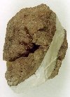
The Lystrosaurus.
The Lystrosaurus encapsulated in rock.
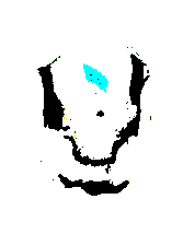
2D CAT scanned slice Nr. 138
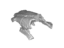
3D rendering of the top twenty slices

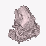
3D rendering of the skull
3D rendering of the skull
Lystrosaurus - A Therapsid (mammal-like reptile) that was present in very large numbers (running into the millions) in Gondwana during the Triassic period. (Gondwana was the supercontinent consisting of the landmasses of South America, Africa, Antarctica, Australia and India that split and drifted apart during the periods following the Triassic.) It is a member of a group of therapsids called Dicynodonts, characterized by their horny beaks and only two teeth - the canines, which grew quite large and appeared like tusks. They lived in sizable herds beside water sources (rivers and lakes), and were herbivorous. Probably the major component of their diet consisted of plants called horsetails, which grew more than a meter tall. Lystrosaurus are particularly interesting because they were among the few Dicynodonts to appear in the fossil record after the great extinction event at the end of the Permian period, which wiped out 95 percent of all life on earth. In fact, the Lystrosaurs were present with the first dinosaurs. There were at least two species of Lystrosaur: a very large one with a flat-fronted face that grew to the size of a big Brahman bull, and a smaller one with a more rounded snout. They were sprawling animals, chunky and lumbering and probably incapable of any great burst of speed. They would not have been scaly or furry, but would have had tough leathery skins. Lystrosaurus are creatures that inhabited the ancient Karoo area of South Africa.
Pronunciation guide: Lystrosaurus (Liss- tro- SAW- russ) Dicynodont (Dy-SY-no-dont) Gondwana (Gone-DWA-na) Triassic (Try-ASS-ik) Permian (PUR-mee-un). [15]
The Permian started around about (approximately and all that) 286 million years ago and ended with the start of the Triassic about 248 million years ago. Your first dinosaurs therefore pitched up about the middle of the Triassic (220 million years ago or so).
The Materialise software was applied extensively during the conversion
process. This was a very interesting case study. What made it so interesting
was that the fossil’s skull was and is still encapsulated in rock. The
big advantage is that the rock can now be electronically removed to display
the fossil, with the aid of CAT and 3D computer image processing. The cost
and time saving are astronomically. Imagine an archeologist spending months
to grind the rock away, compared to this new process that will take less
than a week. This fossil was scanned at two hospitals, Hydromed and Krugersdorp
Private Hospitals. Different apparatus was used hoping to get better results
from the more recent spiral CAT scanners.
Referring to the following data sheet, the fossil’s skull can be retrieved from the rock in about 14 hours and costs about R2400 excluding CAT scanning. 3D renderings can be supplied at this stage. 3D data is also available, virtual reality programs can be used to realistically visualize the fossil. Another estimated R2000 and two days will allow one to produce a 3D physical prototype. Compare this with the conventional method, taking several weeks to extract the fossil from the rock. There may not be a great cost saving at this stage. With this method, one can very quickly determine what is inside the rock. Several weeks may be spent extracting the fossil from the rock and the fossil may not be of great value or importance. It will therefore streamline the process. Making use of this technology will enable the anthropologist to be effective and efficient.
4.1.2.1 Images
|
|
| Figure 4.1.2
.1
The Lystrosaurus. |
Figure 4.1.2
.2
The Lystrosaurus encapsulated in rock. |
|
|
|
| Figure 4.1.2
.3
2D CAT scanned slice Nr. 138 |
Figure 4.1.2
.4
3D rendering of the top twenty slices
|
|
|
| Figure 4.1.2
.5
3D rendering of the skull |
Figure 4.1.2
.6
3D rendering of the skull |
| Description | Options (Default) | Data
K’dorp |
Data Hydromed | |
| 1 | CT Image Names | fos.xxx | 4s4I | |
| 2 | Patient/Project Name | fos.pat | 4s4i.pat | |
| 3 | Number of First Input Image | 27/01 | 68 | |
| 4 | Number of Last Input Image | 157/99 | 133 | |
| 5 | Number of First Output Image | 000 | 000 | |
| 6 | CT or MRI | CT, MRI | CT | CT |
| 7 | Horizontal Nr. Of Image Pixels | 0 to 65535 (265,512,1024) | 512 | 512 |
| 8 | Vertical Nr. Of Image Pixels | 0 to 65535 (265,512,1024) | 512 | 512 |
| 9 | Number of Images per File | (1) | 1 | 1 |
| 10 | File Swap Format (0,3) | 0,3 | CCELSC | CCGEADVA |
| 11 | Pixel Type | B,UB,S,US,L,UL,F | - | - |
| 12 | Header Size | *see formula below | - | - |
| 13 | Inter Image Header Size | 0 | - | - |
| 14 | Add Value | 0 to 4095 | - | - |
| 15 | Scale Value | 0 to 4095 | - | - |
| 16 | Table Position | (mm) | 0 | 0 |
| 17 | Distance Between Slices | (mm) | 1 | 1 |
| 18 | Slice thickness | (mm) | 1 | 1 |
| 19 | Pixel Size SQ. | F.O.R./Nr. Hor. Pixels (mm) | 0.47 | 0.43 |
| 20 | Gantry Tilt Angle | Degrees | 0 | 0 |
| 21 | Field of Reconstruction/View | (mm) | 240 | 220 |
| 22 | Number of Images | 130 | 65 | |
| 23 | File Size of CAT Image | Kb | 270-280 | 270-280 |
| 24 | File Size of Converted Image | Kb | 135 | 135 |
| 25 | .3dd file size | Mb | 1.4 (X.srf) | 1.4 (X.srf) |
| 26 | .STL file size | Mb | not grown | Not grown |
| 27 | RP Method | (SLA,FDM,OTHER) | - | - |
| 28 | .IGS file size | Mb | - | - |
| 29 | RP Slice file size | Mb | - | - |
| 30 | RP Download File size | Mb | - | - |
| 31 | Grow Time | Hour | - | - |
| 32 | Tip size | (T12, T25) | - | - |
| 33 | Slice Thickness | (0.01", 0.014") | - | - |
| 34 | Finishing Time | Hour | - | - |
| 35 | Processing Time | Hour | 5 | 10 |
| 36 | Data Retrieval Time | Hour | 4 | 4 |
| 37 | Total Cost | Rand | =14*150+300
=2400 |
