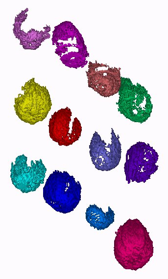
Isometric view of several avocado’s water rich areas.
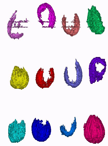
Front view of several avocado’s water rich areas.
This case study was performed for a group of the CSIR’s food technologists. The study was based on a similar case that was performed in the USA with nuts. The aim of this study was to separate the fat rich areas from the water rich areas within the avocado. The separation is normally done by destroying the avocado in order to determine the stage of ripeness. The food technologists hoped to develop a non-destructive evaluation method to determine the ripeness of the avocado. This same process can then be used to analyze other fruit such as mangos.
The avocados were marked and placed in fixture. Avocados
at different stages of ripeness were selected.
Pretoria East Hospital was again approached to perform the CAT scanning. . A series of axial sections were produced. The data was retrieved and converted. The next step was to separate the fat-rich areas from the water-rich areas. The water rich areas were the regions of interest.
Every material has certain properties. Digital images
are produced as a result of the CAT scanning. These digital images consist
of pixels. Each pixel represents a part of the component that is scanned.
The pixels are also made up of different Grey scale values, better known
as the Hounsfield unit. This phenomenon was used to separate the water
rich areas from the fat rich areas. Pure water’s Hounsfield unit is 1000
while that of air is 0. The Hounsfield theory is described in the Basic
Principals of CAT. Separation was achieved by setting the bandwidth of
the threshold to approximately 1000 Hounsfield units. A 10 units tolerance
band was used.
This unique method was successfully applied to supply the food technologists with results. Again, this method proved to be the only non-destructive method to perform the analysis.
The volumes and areas of dispersion were determined for
every avocado of the water rich areas as well as the complete avocado.
The food technologists further manipulated the data that showed a clear
trend. This process proved to be helpful towards the predicament of the
avocado’s ripeness. Avocados could be scanned on a routine basis where
the ideal ripeness stage could be predicted. Environmental influences had
to be taken into account during the predicament. This case study opened
a brand new field of application for this wonderful unique combination
of technologies. Biological applications can now be added to the medical,
industrial and fossil related fields of applications. The following table
will list the mass and volumetric data.
Table 4.15.2 – Avocado Mass & Volumetric Data
4.15.2.1 Images
|
|
| Figure 4.15.2.1
Isometric view of several avocado’s water rich areas. |
Figure 4.15.2.2
Front view of several avocado’s water rich areas. |
| Description | Options (Default) | Data
|
|
| 1 | CT Image Names | Avos.00 | |
| 2 | Patient/Project Name | Avos.pat | |
| 3 | Number of First Input Image | 212 | |
| 4 | Number of Last Input Image | -254 | |
| 5 | Number of First Output Image | 000 | |
| 6 | CT or MRI | CT, MRI | CT |
| 7 | Horisontal Nr. Of Image Pixels | 0 to 65535 (265,512,1024) | 512 |
| 8 | Vertical Nr. Of Image Pixels | 0 to 65535 (265,512,1024) | 512 |
| 9 | Number of Images per File | (1) | 1 |
| 10 | File Swap Format (0,3) | 0,3 | 0 |
| 11 | Pixel Type | B,UB,S,US,L,UL,F | Toshiba |
| 12 | Header Size | *see formula below | - |
| 13 | Inter Image Header Size | 0 | - |
| 14 | Add Value | 0 to 4095 | - |
| 15 | Scale Value | 0 to 4095 | - |
| 16 | Table Position | (mm) | -254 |
| 17 | Distance Between Slices | (mm) | 3 |
| 18 | Slice thickness | (mm) | 3 |
| 19 | Pixel Size SQ. | F.O.R./Nr. Hor. Pixels (mm) | 0.7 |
| 20 | Gantry Tilt Angle | Degrees | 0 |
| 21 | Field of Reconstruction/View | (mm) | 380 |
| 22 | Number of Images | 150 | |
| 23 | File Size of CAT Image | kb | 521 |
| 24 | File Size of Converted Image | kb | 10-40 |
| 25 | .3dd file size | Mb | 2.5 ea. |
| 26 | .STL file size | Mb | - |
| 27 | RP Method | (SLA,FDM,OTHER) | - |
| 28 | .IGS file size | Mb | - |
| 29 | RP Slice file size | Mb | - |
| 30 | RP Download File size | Mb | - |
| 31 | Grow Time | Hour | - |
| 32 | Tip size | (T12, T25) | - |
| 33 | Slice Thickness | (0.01", 0.014") | - |
| 34 | Finishing Time | Hour | - |
| 35 | Processing Time | Hour | 5 |
| 36 | Data Retrieval Time | Hour | 4 |
| 37 | Total Cost | Rand | =9*100+300=1200 |

Reverse Engineering Case Studies
Shortcuts back to:
Medical
Studies or
Industrial
& Biological Studies or
Fossil
Studies
or (Back to the Home Page)